| SF Project Page | Frequently Asked Questions |
| About the Project |
| Home page |
| Background |
| Documentation |
| Applications |
| Reviews/Quotes |
| Developers |
| Related |
| Donate |
| Platforms |
| Windows |
| Unix/Linux |
| Mac OS |
| Getting the code |
| Releases |
| Subversion access |
| Contact Us |
| Contact details |
|
|
Background Reading
Theory
Sharpen your pencils, this is the mathematical background (such as it is).- The paper that started the ball rolling: Paul Graham's A Plan for Spam.
- Gary Robinson has an interesting essay suggesting some improvements to Graham's original approach.
- Gary Robinson's Linux Journal article discussed using the chi squared distribution.
more links? mail anthony@interlink.com.au
Overall Approach
Please note that I (Anthony) am writing this based on memory and limited understanding of some of the subtler points of the maths. Gentle corrections are welcome, or even encouraged.
Tokenizing
The architecture of the spambayes system has a couple of distinct parts. The first, and most obvious, is the tokenizer. This takes a mail message and breaks it up into a series of tokens (words). At the moment it splits words out of the text parts of a message, stripping out various HTML snippets and other bits of junk, such as images. In addition, there's a variety of mail header interpretation and tokenization that goes on as well. The code in tokenizer.py and the comments in the Tokenizer section of Options.py contain more information about various approaches to tokenizing, as well as various things that have been tried and found to make little or no difference.
Because the original tests of the system mixed a ham corpus from a high-volume mailing list with a spam corpus from a different source, email header lines were ignored completely at first (they contained too many consistent clues about which source a message came from). As a result, this project tried much harder than most to find ways to extract useful information from message bodies. For example, special tokenizing of embedded URLs was one of the first things tried, and instantly cut the false negative rate in half. In the end, testing showed that very good classifiers can be gotten by looking only at message bodies, or by looking only at message headers. Looking at both does best, of course.
Tokenizing of headers is an area of much experimentation. Unfortunately the only current source of historical information about previous experiments is in the source code, as comments, or in the mailing list archives. At the moment, a bunch of email headers are broken apart, and tagged with the name of the header and the token. Recipient (to/cc) headers are broken apart in a variety of ways - for instance, we count the number of recipients, and generate a token for the nearest power of two to the number. Optionally, "Received" lines are parsed for various tokens.
It's likely that remaining "easy wins" in the tokenizing are buried in some new way of tokenizing the headers. If you have ideas, try them out, and test them. For instance, no-one's tried generating a token that measures the difference in the time in the Date: header, and the time that the message arrived at the user's mailbox.
Another issue that cropped up quite quickly was that certain types of clues were highly correlated. For instance, if the message was a HTML spam, you'd get things like "font", "table", "#FF0000" and the like. This caused any other HTML spam to be marked solidly as spam, but also unnecessarily penalized the non-spam HTML messages. In the end, the best results were found by stripping out most HTML clues.
Combining and Scoring
The next part of the system is the scoring and combining part. This is where the hairy mathematics and statistics come in.
Initially we started with Paul Graham's original combining scheme - a "Naive Bayes" scheme, of sorts - this has a number of "magic numbers" and "fuzz factors" built into it.
The Graham combining scheme has a number of problems, aside from the magic in the internal fudge factors - it tends to produce scores of either 1 (definite spam) or 0 (definite ham), and there's a very small middle ground in between - it doesn't often claim to be "unsure", and gets it wrong because of this. The following plot shows the problem:
Note:In each of these plots, the X axis shows the 'score' of the message, scaled to 0-100. (where 0 is "definitely ham", and 100 is "definitely spam"), and the Y axis shows the number of messages with that score (scaled logarithmically). Note also that the plots aren't from the same data set :-( but are "typical" plots that you'd see from a given technique. One day, if I have enough time, I'll go back and re-do all the plots using a single fixed data set.
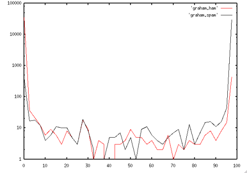
In this plot, you can see that most of the spam gets scores near to 100, while most of the ham gets scores near to 0. This is all good. Unfortunately, there's also a significant number of hams that score close to 100, and spams close to 0 - which means the system is not just scoring them wrong, but it's completely confident in its (wrong) score. (Note that the difference isn't as apparent as it could be - it's a logarithmic scale graph!)
Gary Robinson's essay turned up around this time, and Gary turned up on the mailing list a short time after that.
Gary's initial technique produced scoring like this plot:
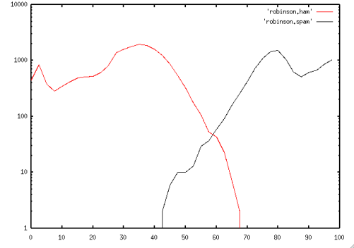
This produces a very different result - but this plot shows a different issue - there's a large overlap between the ham scores and spam scores. Choosing the best 'cutoff' value for "everything higher than this is spam" turned out to be an incredibly delicate operation, and was highly dependent on the user's data.
There's a number of discussions back and forth between Tim Peters and Gary Robinson on this subject in the mailing list archives - I'll try and put links to the relevant threads at some point.
Gary produced a number of alternative approaches to combining and scoring word probabilities. The initial one, after much back and forth in the mailing list, is in the code today as 'gary_combining', and is the second plot, above. Gary's next suggestion involved a couple of other approaches using the Central Limit Theorem (or this, for the serious math geeks).
The Central Limit combining schemes produced some interesting (and surprising!) results - they produced two internal scores, one for ham and one for spam. This meant it was possible for them to return a "I don't know" response, when ham and spam scores were both very low or both very high. This caused some confusion as we tried to map these results to a Graham-like score.
An example: a message with internal spam score that's 50 standard deviations on the spam side of the ham mean score and an internal ham score that's 40 standard deviations on the ham side of the spam mean would, if you just combine them in a straightforward manner, produce a result that it's definitely a spam. But look at the internal scores - it was certain that it wasn't spam, and it wasn't ham, either. In other words, it's not like anything it's seen before - so the only thing to do is to punt it out with an 'unsure' answer.
The central limit approaches were dropped after Gary suggested a novel but well-founded combining scheme using chi-squared probabilities. Tim implemented it, including a unique routine to compute -2*sum(ln p_i) without logarithms and without underflow worries. Many, many testers reported excellent results. This is now the default combining scheme. Some end cases were improved when Rob Hooft discovered a cleaner way to combine the internal overall ham and spam scores, which improved detection of the "middle ground".
Chi-combining is similar to the central limit approaches, but it doesn't have the annoying training problems that central limit approaches suffered from, and it produces a "smoother" score.
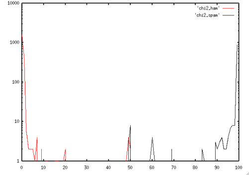
The chi-squared approach produces two numbers - a "ham probability" ("*H*") and a "spam probability" ("*S*"). A typical spam will have a high *S* and low *H*, while a ham will have high *H* and low *S*. In the case where the message looks entirely unlike anything the system's been trained on, you can end up with a low *H* and low *S* - this is the code saying "I don't know what this message is". Some messages can even have both a high *H* and a high *S*, telling you basically that the message looks very much like ham, but also very much like spam. In this case spambayes is also unsure where the message should be classified, and the final score will be near 0.5. The following plot shows this quite clearly. It also shows the quite dramatic results we get from this technique.
So at the end of the processing, you end up with three possible results - "Spam", "Ham", or "Unsure". It's possible to tweak the high and low cutoffs for the Unsure window - this trades off unsure messages vs possible false positives or negatives. In the chi-squared results, the "unsure" window can be quite large, and still result in very small numbers of "unsure" messages.
A remarkable property of chi-combining is that people have generally been sympathetic to its "Unsure" ratings: people usually agree that messages classed Unsure really are hard to categorize. For example, commercial HTML email from a company you do business with is quite likely to score as Unsure the first time the system sees such a message from a particular company. Spam and commercial email both use the language and devices of advertising heavily, so it's hard to tell them apart. Training quickly teaches the system all sorts of things about the commercial email you want, though, ranging from which company sent it and how they addressed you, to the kinds of products and services it's offering.
Training
Training is the process of feeding known ham and spam into the tokenizer to generate the probabilities that the classifier then uses to generate it's decisions. A variety of approaches to training have been tried - things that we found:
- the system generates remarkably good results on very few trained messages, although obviously, the more the better.
- training on an extremely large number of messages may start to produce slightly poorer results (once you're training on thousands and thousands of messages).
- imbalance between the number of ham and spam trained can cause problems, and worse problems the greater the imbalance; the system works best when trained on an approximately equal number of ham and spam.
- It's really important that you're careful about selecting your training sets to be from the same sources, where-ever possible. Several people got caught out by training on current spam, and old ham. The system very quickly picked up that anything with a 'Date:' field with a year of 2001 was ham. If you can't get ham and spam from the same source, make sure the tokenizer isn't going to pick up on the non-clues.
- There is much more discussion about training on the wiki.
Testing
One big difference between spambayes and many other open source projects is that there's a large amount of testing done. Before any change to the tokenizer or the algorithms was checked in, it was necessary to show that the change actually produced an improvement. Many fine ideas that seemed like they should make a positive difference to the results actually turned out to have no impact, or even made things worse. About the only "general rule" that kept showing up was Stupid beats smart. That is, a fiddly and delicate piece of tokenization magic would often produce worse results than something that just took a brute force "just grab everything" approach.
The testing architecture has been in place since the start of the project. The most thorough test script is Tim's cross validation script, timcv.py. This script takes a number of sets of spam and ham. It trains on all but the first set of spam and ham, then fires the first set of spam and ham through, and checks how it goes at rating them. It then repeats this for each set in turn - train on all but the set being tested, then test the set.
Mailing list archives
There's a lot of background on what's been tried available from the mailing list archives. Initially, the discussion started on the python-dev list, but then moved to the spambayes list.
- The fun started in August 2002. thread 1, thread 2.
- But wait, there's more! In the September archive, thread 1, thread 2, thread 3, thread 4, thread 5.
- The discussions then moved to the spambayes mailing list.
CVS Commit Messages
Tim Peters has whacked a whole lot of useful information into CVS commit messages. As the project was moved from an obscure corner of the Python CVS tree, there are actually two sources of CVS commits.
- The older CVS repository via view CVS, or the entire changelog. Development here stopped on the 6th of September 2002.
- After that, work moved to this project's CVS tree
Papers about SpamBayes
Tony Meyer and Brendon Whateley wrote a